MSc Big Data Analytics · Dissertation Defense

Unsupervised Discovery of
Urban Mobility Archetypes

Six unsupervised layers. 19.5 million NYC taxi trips. One city's hidden rhythm.

Rubin Apore•Student ID 22495624

→ / space to advance · F for fullscreen

Roadmap

What we'll cover

01

Motivation & gap

02

Research questions

03

Data & scale

04

Six-layer pipeline

05

Spatial archetypes

06

Temporal rhythms

07

Spatiotemporal fingerprint

08

Anomalies

09

Unified embedding

10

Cross-method triangulation

11

Validation & rigor

12

Theoretical grounding

13

Limitations & ethics

14

Contribution

15

Future work

Every method section pairs what we found with why that method, and not another.

Motivation

Every taxi trip is a tiny decision.
Millions of them reveal how a city moves.

Most NYC taxi research stops at demand prediction or hotspot detection. Far fewer derive interpretable, validated mobility archetypes that hold up across spatial, temporal, and behavioural dimensions at once.

That's the gap this project targets: not "where do people go", but "what recurring types of mobility behaviour exist, and can we prove it?"

Research Questions

Five questions, five pipeline layers

Layer 1 (load, clean, feature-engineer) underpins all five: it doesn't answer one RQ on its own, so RQ1 begins at Layer 2.

RQ1

What distinct spatial demand archetypes emerge across NYC's 260 active taxi zones? · Layer 2

RQ2

How do temporal rhythms differ across zones? · Layer 3

RQ3

What latent spatiotemporal structure jointly explains zone × hour × day-type behaviour? · Layer 4

RQ4

Which trips/zones behave anomalously, and why? · Layer 5

RQ5

Can every zone be reduced to one unified, interpretable fingerprint? · Layer 6

Data & the Big-Data Problem

NYC TLC Yellow Taxi · Jan–Jun 2023

19.5M

raw trips

95.8%

retained after QC

260

of 263 zones active

500K

unbiased trip-level sample

The big-data constraint is real, not decorative: Layer 1 streams through six monthly Parquet files one at a time, computing exact zone-level and tensor aggregates incrementally, the full 19.5M rows are never materialised in memory at once. A fixed random seed (42) runs through every stochastic step.

Why · Layer 1 Engineering Decision

Why streaming, not full materialisation

  • ▸ The originally proposed approach (load all 18.68M filtered rows into one DataFrame) was estimated at >2.5GB in memory, before any modelling even starts.
  • ▸ Instead, each of the 6 monthly Parquet files is loaded, filtered, and feature-engineered in turn, then folded into three compact running artefacts before being discarded:
  • · per-zone aggregate sums (zone-level means/shares derived once all months are processed)
  • · a Zone × Hour × Day-type trip-count tensor (built incrementally, exactly, not sampled)
  • · a proportionally-sampled ~500K-trip subset retained for Layer 5
  • ▸ Result: peak memory is bounded to one month's frame (~3M rows) regardless of how many months are added: genuinely bounded growth, not just "a script that happens to use a big file."

Methodology

The six-layer pipeline

L1

Load & clean

L2

K-Means
spatial

L3

K-Shape
temporal

L4

Tucker
joint

L5

Isolation Forest
anomaly

L6

UMAP
fingerprint

Each layer answers one research question independently, then Layer 6 fuses their outputs into a single 260-zone fingerprint, deliberately comparing multiple paradigms rather than committing to one clustering method up front.

Layer 2 · RQ1

Spatial demand archetypes

  • 🟡 High-volume Manhattan core: 53 zones, 15.8M trips, $16.91 avg fare
  • 🌙 Nightlife / entertainment: 19 zones, 48.7% night trips, 56.4% weekend
  • ✈️ Airport / transport hub: 47 zones, $51.15 avg fare, 12.3mi avg
  • 🏘️ Outer-borough residential: 85 zones, low cash & weekend share
  • 💵 Mixed-access: 56 zones, elevated cash share (28.1%)

k = 5 chosen for interpretability: the statistical optimum (k = 2, silhouette 0.307) collapses everything into two uninformative groups.
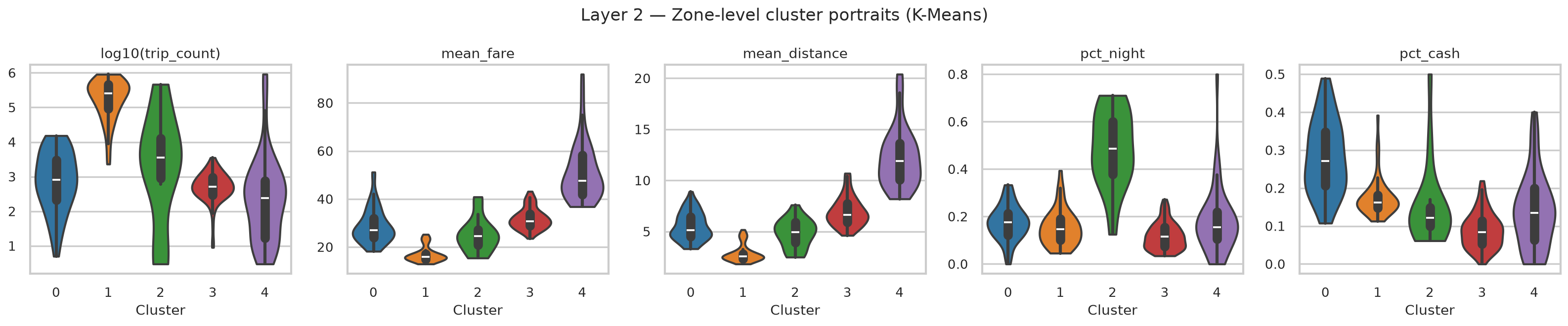
K-Means cluster fare/distance violin plots Details ↗

Why · Layer 2 Method Justification

Why K-Means, and why not something else

  • ▸ 10-feature, z-score standardised zone profile (log trip count, mean fare/distance/duration/speed, tip share, weekend/cash/night/rush shares): Euclidean distance assumes roughly spherical clusters in this standardised space.
  • ▸ The silhouette curve is comparatively flat (0.264–0.307 across k = 2–8), with no sharp elbow. The k = 2 global peak is driven almost entirely by airport zones separating from everything else.
  • ▸ k = 5 was adopted using the proposal's own pre-registered validation criterion (interpretability against known NYC geography) for a modest 0.019 silhouette cost. Both solutions are reported for transparency, not just the one that "won."

Acknowledged limitation: K-Means assumes convex, similarly-sized clusters, but NYC's zone geometry is irregular, so DBSCAN is flagged as future work precisely because it doesn't share that assumption.

K-Shape temporal rhythm centroids Details ↗

Layer 3 · RQ2

Temporal rhythms

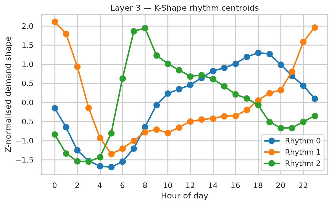
99 zones with sufficient hourly signal · best k = 3 (silhouette 0.355)

  • Evening / business-dominant: 62 zones, peaks 18:00, mostly Manhattan
  • Nightlife (midnight-peaking): 14 zones, peaks 00:00, Brooklyn-leaning
  • Morning-commuter: 23 zones, peaks 08:00, outer-borough mix

Why · Layer 3 Method Justification

Why K-Shape, and why normalise twice

  • ▸ K-Shape (Paparrizos & Gravano, 2015) clusters on a shift-invariant, cross-correlation-based shape distance: built for exactly this question: do rhythms match in shape, regardless of when the pattern begins.
  • ▸ Two-stage normalisation: raw hourly counts → fractional hourly share (removes the effect of absolute volume), then z-normalise the resulting shape (removes offset and scale). A low-volume residential zone peaking at 8am now clusters with Midtown, which also peaks at 8am. This is intentional, since RQ2 asks about rhythm, not scale.
  • ▸ Zones averaging fewer than 10 trips/day were excluded first (leaves 99 of 260 zones), to prevent sparsity-induced shape distortion.

Honest caveat: K-Shape's native shape distance isn't compatible with the standard silhouette formula, so k was selected via silhouette on Euclidean distance between the same z-normalised shapes: a documented approximation, not the native metric.

Layer 4 · RQ3

Non-negative Tucker decomposition

A Zone × Hour × Day-type tensor, factorised at rank (6, 4, 2): 98.2% explained variance, reconstruction error 0.134.

4 hour-mode components (peak times)

  • Evening rush: peaks 18:00
  • Morning rush: peaks 08:00
  • Late-night: peaks 23:00
  • Midday: peaks 15:00

6 independent zone-mode components (top-loading zones)

Midtown East/Penn Station, East/West Village, Times Sq/JFK, Midtown Center/Union Sq, Upper West Side, and Upper East Side/LaGuardia each dominate their own component: recognisable neighbourhood groupings, not tied 1:1 to the hour components above.
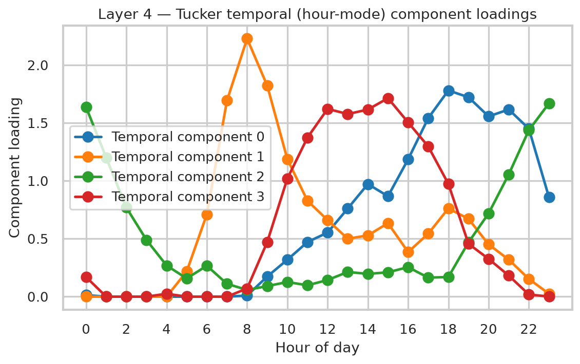
Tucker hour component factors Details ↗

Why · Layer 4 Method Justification

Why Tucker, not a 2D matrix factorisation

  • ▸ Demand is inherently three-dimensional: zone × hour × day-type. A matrix factorisation (e.g. NMF) must first collapse one mode, losing that interaction structure. Tucker (Kolda & Bader, 2009) preserves all three modes simultaneously.
  • ▸ Non-negativity enforced throughout: demand cannot be negative, and it makes component loadings directly interpretable as "how much of this pattern," not abstract signed weights.
  • ▸ Random, not SVD, initialisation for the multiplicative-update algorithm. SVD init was found empirically to diverge (numerical overflow) at this tensor's scale. A real engineering finding, not a default choice.
  • ▸ Rank (6, 4, 2) was retained even though the neighbouring rank (5, 4, 2) achieves marginally lower reconstruction error (0.117 vs 0.134), which is expected under non-convex multiplicative-update optimisation converging to different local minima, not evidence against (6, 4, 2), which was kept for its finer zone-mode resolution.
Isolation Forest zone anomaly heatmap Details ↗

Layer 5 · RQ4

The 2% that don't fit the pattern

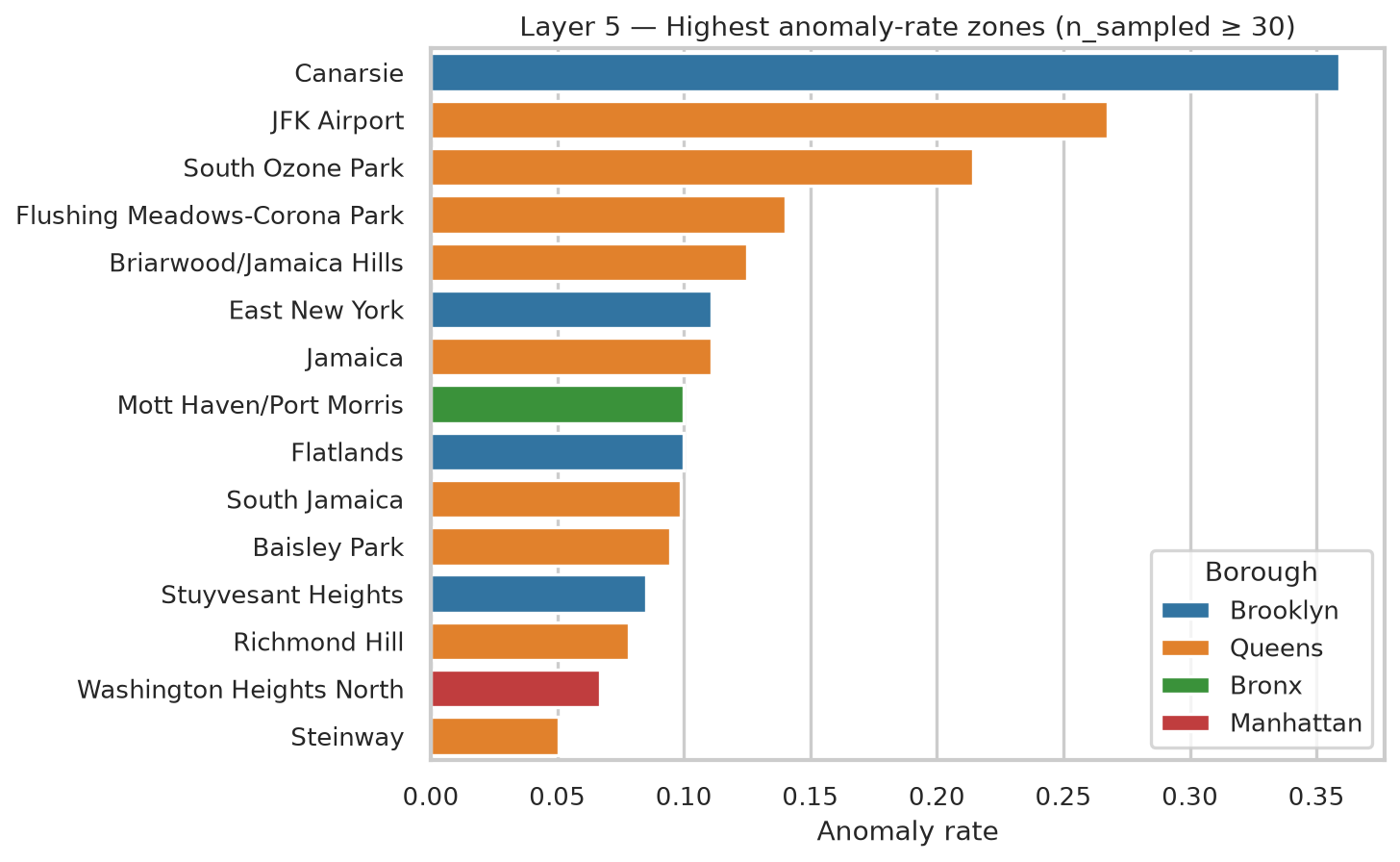
10,000 of 500K sampled trips flagged anomalous, not fraud, but long, fast, expensive outliers:

$70 vs $12.80

fare

18.8mi vs 1.8mi

distance

27mph vs 10mph

speed

Top anomaly zones: Canarsie (36%), JFK Airport (27%), South Ozone Park (21%).

Why · Layer 5 Method Justification

Why Isolation Forest, and what it doesn't claim

  • ▸ Isolation-based, not distance- or density-based: anomalies are isolated by random recursive partitioning in fewer splits: no distance metric required, near-linear scaling, well suited to mixed-scale tabular trip features.
  • ▸ 200 trees, 2% contamination, a 7-feature input (distance, duration, fare, speed, tip %, hour, weekend), fit on the 499,998-trip representative sample.
  • ▸ Explicit epistemic framing: this layer does not prove fraud; it flags structurally unusual trips that may warrant compliance review, nothing more.

Reference-class caveat: the model is trained on the pooled, Manhattan-dominated trip distribution, so "anomalous" partly reflects distance from that norm (e.g. airport trips), not proof of misconduct. Worth stating explicitly before handing a ranked list to a regulator.

Layer 6 · RQ5

One fingerprint per zone

All 260 zones reduced to a 17-dimensional fingerprint (volume, fare, speed, tip %, cash/night/weekend share, six Tucker zone factors, anomaly rate), then embedded in 2D with UMAP.

Linear PCA explains only 48.8% of variance in 2D. UMAP preserves local neighbourhood structure instead, revealing a continuous archetype gradient rather than hard boundaries, echoing, and sharpening, the Layer 2 clusters.
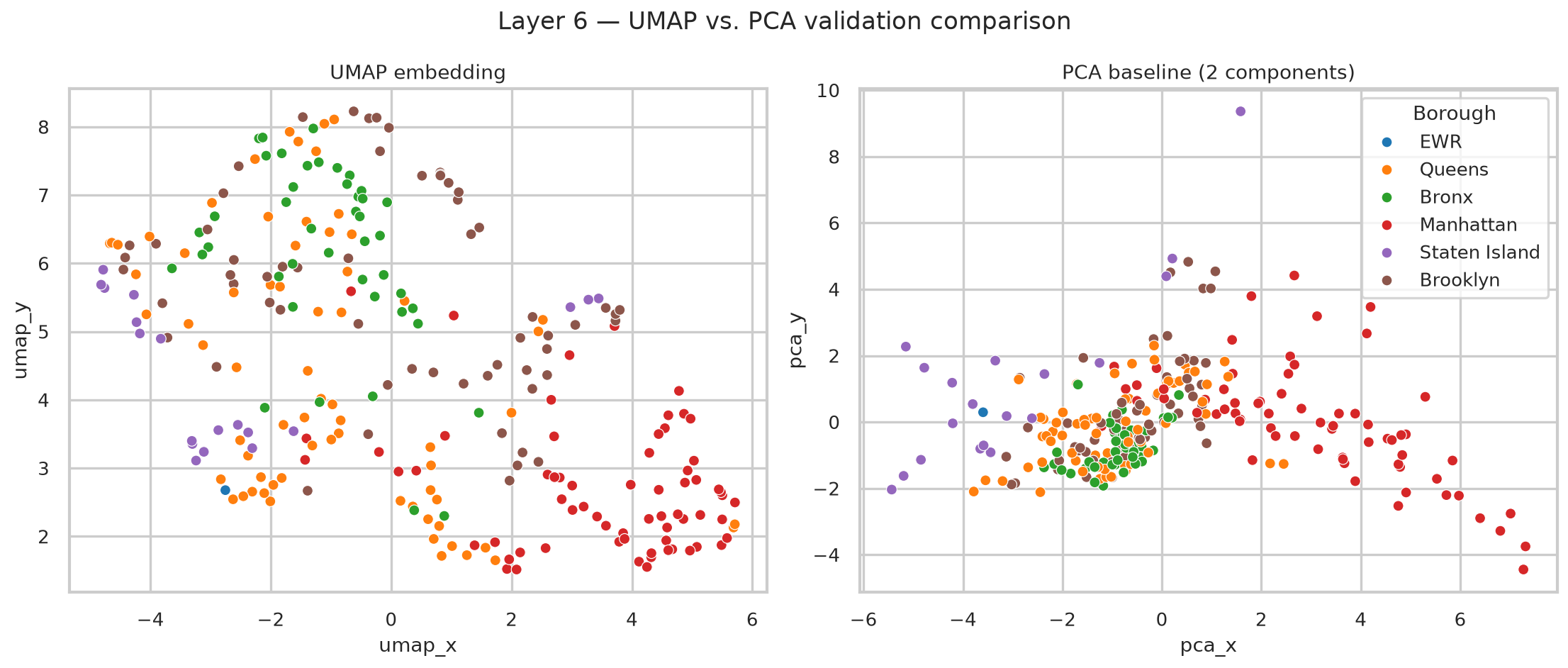
UMAP vs PCA zone embedding comparison Details ↗

Why · Layer 6 Method Justification

Why UMAP, and why treat it as exploratory

  • ▸ UMAP (McInnes, Healy & Melville, 2018), n_neighbors=10, min_dist=0.25: preserves local neighbourhood structure via fuzzy topological approximation, rather than global variance (PCA) or purely local density with no global-structure guarantee (t-SNE).
  • ▸ The PCA baseline on the same 17-D fingerprint explains only 48.8% of variance in 2D: direct quantitative evidence the fingerprint's structure is meaningfully non-linear, justifying manifold learning over a linear projection.

Explicitly used as an exploratory visualisation tool, not a confirmatory statistical test; UMAP inter-cluster distances are not globally meaningful, so no statistical claims are drawn from embedding geometry alone; it's validated instead against Layer 2's cluster labels and known borough membership.

Discussion

Independent methods, convergent findings

  • ▸ K-Shape (shape-based time-series clustering) and Tucker (tensor factorisation) each independently recover a nightlife/midnight-peaking pattern, via completely different mathematical machinery. Convergence across independent methods is stronger evidence than either method alone.
  • ▸ Tucker's weekday-only day-type component (loading 0.37 weekday vs ≈0.0003 weekend) has no analogue in K-Means or K-Shape: a genuinely latent pattern visible only because the full three-mode tensor structure was preserved rather than collapsed.
  • ▸ The UMAP fingerprint recovers NYC's borough geography with no borough labels ever supplied to the model: the strongest evidence that all four preceding layers measure one coherent underlying reality, not four unrelated sets of clusters.

Validation & Rigor

One score is never enough

Multi-k comparison

Silhouette curves computed for k = 2–8 (L2) and 2–6 (L3), not a single arbitrary choice.

Interpretability over pure optimum

k = 5 chosen over statistically "best" k = 2: justified, not defaulted.

Rank sensitivity

Tucker rank (6,4,2) checked against three alternative ranks before committing.

Stability testing

Isolation Forest anomaly rates correlate 0.55 across random data halves.

Theoretical Grounding

Why unsupervised learning, why this literature

Big Data 5 Vs (Laney, 2001)

★★★★★

Volume

★★★★

Velocity

★★★★

Variety

★★★

Veracity

★★★★★

Value

  • ▸ Urban informatics / Smart City paradigm (Batty, 2013): taxi records are a canonical urban-informatics dataset: city-scale mobility behaviour without GPS-level privacy cost.
  • ▸ Unsupervised learning as hypothesis generation (Tukey, 1977; Hastie et al., 2009): the goal is discovering which hypotheses are worth testing next, not confirming one pre-specified outcome.
  • ▸ Tensor methods in urban analytics (Kolda & Bader, 2009; Cichocki et al., 2016): the mathematical foundation for Tucker decomposition and for non-negativity as a route to interpretability.

Literature Positioning

Where this sits in the literature

  • ▸ Yuan et al. (2011) predict zone-level demand hotspots for a single driver: RQ1 generalises this from a single-driver recommendation problem into a city-wide unsupervised taxonomy.
  • ▸ Castro et al. (2012) model traffic from trip-level GPS traces: this analysis trades that spatial resolution for the privacy and openness of TLC's zone-level, non-GPS release.
  • ▸ Colak et al. (2016) model urban congestion across transport modes via mobile-phone data: motivates the tri-modal (yellow / green taxi / FHV) comparison proposed as future work.
  • ▸ Zheng et al. (2014) survey urban computing broadly: situates taxi analytics as one instance of dense, sensor-generated urban data supporting analysis beyond its original operational purpose.

Limitations

Where this should be read carefully

  • ▸ Zone-level, not GPS-level, spatial resolution: some within-zone blurring
  • ▸ Anomaly stability is moderate (0.55), not high: a few small-sample zones excluded as artefacts
  • ▸ Six months of 2023 only: seasonal and multi-year generalisation untested
  • ▸ Yellow taxis are a small, declining share of NYC mobility relative to app-based FHVs, but remain the only fully open, trip-level dataset at this volume and resolution
  • ▸ Tucker reconstruction leaves 1.8% of variance unexplained: human mobility tensors are inherently noisy; the retained rank captures macro-structure without overfitting to sparse, high-frequency noise
  • ▸ Archetype labels are an interpretive step, grounded in the data but not purely algorithmic

Data Ethics & Privacy

Open, anonymised, and zone-level by design

  • ▸ NYC TLC trip records are published as open government data, anonymised at source: no driver or passenger identifiers are included anywhere in the dataset.
  • ▸ Locations are reported at zone level, not GPS coordinates, preventing re-identification of individual trips.
  • ▸ The anomaly layer identifies trip-level patterns, not individual actors. Any regulatory application would require separate data linkage by the TLC under its own compliance mandate; this research outputs only aggregate, zone-level statistics.

Contribution

A reproducible framework, not just one clustering run

A scalable, streaming, six-layer unsupervised pipeline that turns 19.5M raw taxi trips into an empirically derived, validated taxonomy of NYC mobility behaviour: spatial archetypes, temporal rhythms, a joint spatiotemporal fingerprint, flagged anomalies, and one unified embedding.

Fixed seeds. Explicit validation at every layer. Fully open-sourced.

Future Work

Four natural extensions

  • ▸ Extend to a full year or multiple years (including the COVID-19 disruption) to test whether these archetypes are seasonally stable or specific to January–June.
  • ▸ Incorporate green taxi and For-Hire Vehicle (Uber/Lyft) records for a tri-modal comparison, addressing the yellow-taxi selection bias noted throughout.
  • ▸ Apply DBSCAN as an alternative to K-Means: may better respect NYC's irregular, non-convex zone geometry than a centroid-based method.
  • ▸ Apply the same streaming, multi-layer template to Ghanaian urban transport data as comparable digital-ticketing, ride-hailing, or GPS fleet-tracking records become available: a methodological template, not a New-York-specific result.

Thank you

Questions?

Every trip tells a story. Together, they told us five.

github.com/4barz/nyc-taxi-urban-mobility-archetypes

Appendix: full figure & table reference →
1 / 1